How to Solve Math Problems like Writing Code

Math is hard. For one, many of the concepts are presented very abstractly, which can make it difficult at times to relate to reality. It also has an incredible ability to convert optimism into frustration when your solution to a problem evaporates upon checking it.

Only a year or so ago did I realize that math was more than solving problems on school tests. I was working on a programming project when I began to realize that my code was beginning to intersect with some of the math I was taught in my classes. It was at this point that I defined the problem in more mathematical terms.

The problem can be defined fairly simply: find an equation for a surface which intersects four points in 3D space. If 2 or more of the points are the same this problem becomes trivial. However, no linear surface can intersect four different points in 3D space. This is why video games or other 3D models use what's called a triangle mesh, or a bunch of surfaces between 3 points.

Solving the Problem

The first time I tried to solve this problem I had neither the skills nor the proper math problem-solving skills to do it. I tried using a distance-formula solution and a couple other ineffective solutions. A year later though, I came back to the problem with a different approach. This time, I approached it the same way I would a coding problem rather than a math problem.

Normally speaking, solving a coding problem can be broken into 3 parts. The first is to define the end goal. In math, this would be equivalent to specifically specifying your problem. Next, divide the problem into a series of subproblems, where each subproblem steps toward the solution to the larger problem. You normally break my code into functions or classes, and further down to specifc lines of code. Finally, the last step is to bring all the subproblems together to find a solution to the main problem.

Drawing a Diagram

For me, drawing a diagram helps greatly with the second step of dividing up the problem. A diagram visually represents a problem, which makes identifying different parts of the problem come more naturally. The diagram I drew for this problem is rather simple. I started by drawing 4 points on a paper, and naming them A, B, C, and D.

Now that we have our four points, how can we draw some intuition about how to aproach this problem? For me, this came from the idea that a curve can be made from a lot of lines. In calculus, these lines are called the tangent line. Below you can see this in action:

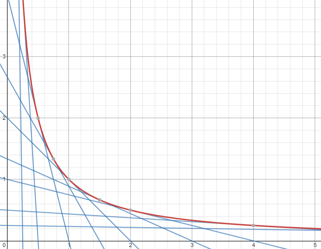
This graph shows how a bunch of straight lines can show the outline of an equation. In this case, the equation in red is \(f(x)=\frac{1}{x}\). To find these lines I took the derivative of this equation, which is \(f'(x)=-\frac{1}{x^2}\), and used that as the slope of each of these lines.

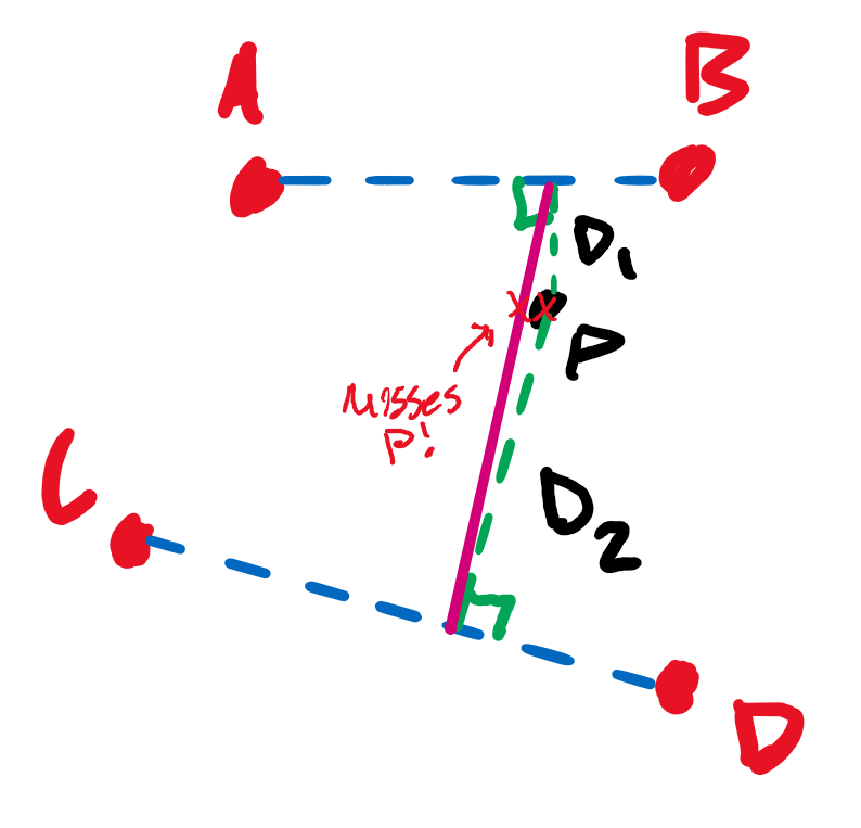
I decided that a similar approach could be used to interpolate 4 points in 3d space. I would take two points and draw a line between them. Then I would draw a line between the two leftover points. From here, we can find a surface that intersects all 4 of the points by dragging a line in which one side intersects the first line we drew and the other intersects the other line where the intersection points on both lines must be of the same ratio between the distance from the starting point and the total length of the drawn lines. This concept isn't very intuative written out, so here's a diagram:

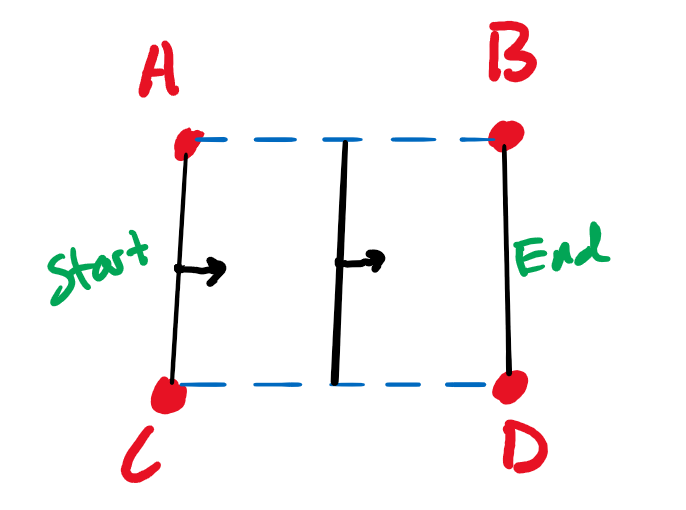
This diagram is 2 dimensional, so each of these points also have some height associated with them. It shows how  you can draw a surface by moving a line from one set of two points to another. The immediate thought is to define this equation parametrically, because there is a notion of time involved here. We could say that \(t=0\) when the black line intersects A and C, and \(t=1\) when it intersects with B and D. This would work fine, but I wanted to solve it directly as a function.

First Subproblem: Measure of Distance

The first subproblem I needed to solve was to find what black line I should use to calculate the height of the surface for any given x and y value. I also wanted this formula to extrapolate beyond the bounds of A, B, C, and D, and given the method outlined in the diagram there is no reason this shouldn't be possible. The first step I took is to find a function that would input x and y coordinates and output some measure of how close we are to a blue dotted line. If we are right on a blue dotted line, then our z coordinate will be that of the blue dotted line at that point. If its somewhere in between. To find this "somewhere in between" value we will simply draw two perpendicular lines, one starting from line AB and the other starting frim line CD.

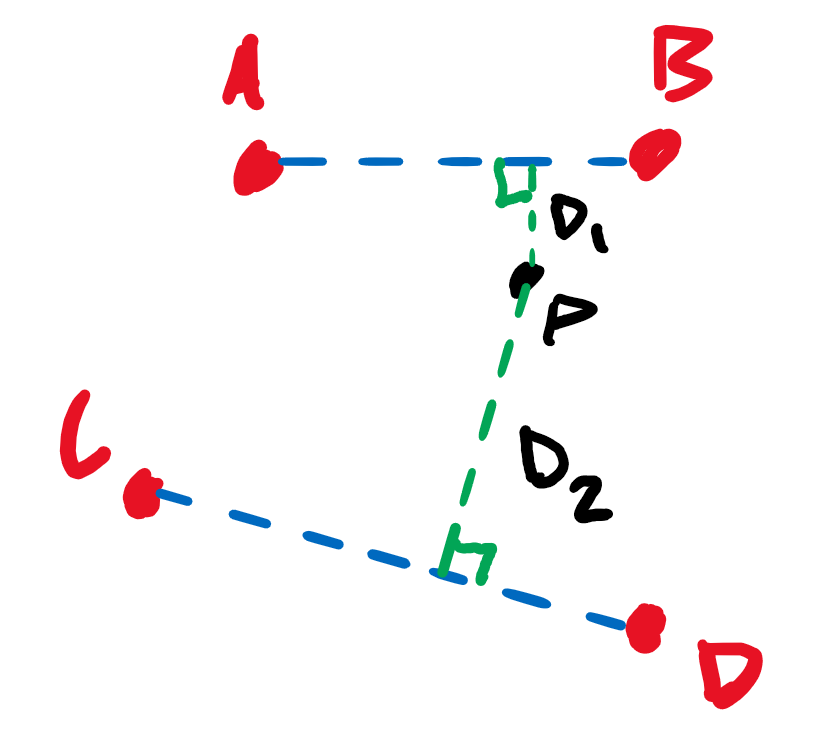
The values \(D_1\) and \(D_2\) are the lengths of these dotted green lines. The reason we make the lines perpendicular is really because it makes the math easier. You could in theory use any angle so long as you kept it consistent between the AB and CD lines, but making it a perpendicular angle makes everything nicer. Now we just have to calculate \(D_1\) and \(D_2\). To do this we will use some vector math. If we take a vector from A to B, written as \(\overrightarrow{AB}\), and project a vector from A to P (the point we are trying to calculate z for), we get a vector pointing to the intersection between the blue and green dashed lines. From there we can subtract that vector from vector \(\overrightarrow{AP}\) and get a vector from the intersection of the blue and green lines to point P. Simply find the magnitude and you get \(D_1\). The same can be done for CD, but replacing every A with a C and every B with a D.

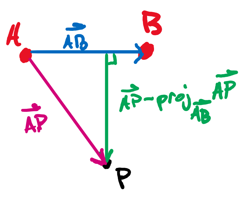
Here are the equations for the functions \(D_1\) and \(D_2\):

\[D_1(P)=||\overrightarrow{AP}-proj_{\overrightarrow{AB}}\overrightarrow{AP}||\] \[D_2(P)=||\overrightarrow{CP}-proj_{\overrightarrow{CD}}\overrightarrow{CP}||\]

Second Subproblem: Finding the proper line intersections

This problem was the most difficult for me. I had to find the distance along \(\overrightarrow{AB}\) and \(\overrightarrow{CD}\) that the black line should intersect with. It would have been convenient to simply use the points we found last time that formed a perpendicular line with point P, but if you draw a line between these two points they aren't guarenteed to intersect with P.

So what do we do? This is exactly why we defined \(D_1\) and \(D_2\) in the first place. In this case, we want to define a function which takes in our x and y coordinate in a vector called P just like as in D, but output a vector pointing to the 2D x and y point in which the black line should intersect with the blue lines. We will call these functions \(P_{ab}\) and \(P_{cd}\). To calculate these values all we have to do is find the total length of \(\overrightarrow{AB}\) and \(\overrightarrow{CD}\) weighted by the ratio between \(D_2\) or \(D_1\) and the sum \(D_1+D_2\) respectively. We have to do a fancy little operation where we multiply our point P elementwise by \(\overrightarrow{AB}\). I will denote this operation with the symbol \(\circ\). This operation performs a similar function to the dot product. We then divide this quantity by the weighted sum of magnitudes discussed earlier. It's perhaps best if you see the equations:

\[P_{ab}(P)=\frac{P\circ\overrightarrow{AB}}{||\overrightarrow{AB}||\frac{D_2(P)}{D_1(P) + D_2(P)}+||\overrightarrow{CD}||\frac{D_1(P)}{D_1(P)+D_2(P)}} + A_{xy}\] \[P_{cd}(P)=\frac{P\circ\overrightarrow{CD}}{||\overrightarrow{AB}||\frac{D_2(P)}{D_1(P) + D_2(P)}+||\overrightarrow{CD}||\frac{D_1(P)}{D_1(P)+D_2(P)}} + C_{xy}\]

Although confusing, this was the biggest step in the problem. Now we can very easily calculate the Z coordinate of this position with the following equations. They look moderately complex but all they are doing is finding a value on a line.

\[Z_{P_{ab}}(P)=(B_z-A_z)\frac{||\overrightarrow{AP_{ab}(P)}||}{||\overrightarrow{AB}||}+A_z\] \[Z_{P_{cd}}(P)=(D_z-C_z)\frac{||\overrightarrow{CP_{ab}(P)}||}{||\overrightarrow{CD}||}+C_z\]

Third Subproblem: Bringing it all together

Now all that's left to do is calculate the Z coordinate on the line for which we know two intersection points for, defined by the functions \(P_{ab}\), \(P_{cd}\), \(Z_{P_{ab}}\), and \(Z_{P_{cd}}\)

\[Z(P)=\left(Z_{P_{ab}}(P)-Z_{P_{cd}}(P)\right)\frac{||\overrightarrow{P_{cd}(P)P}||}{||\overrightarrow{P_{ab}(P)P_{cd}(P)}||}+Z_{P_{cd}}(P)\]

This equation works by essentially making a line of form \(y=mx+b\), where b is the Z coordinate of \(P_{cd}\), and adding the \(mx\) term. The \(mx\) term is made up of the distance \(x\), which is \(\left(Z_{P_{ab}}(P)-Z_{P_{cd}}(P)\right)\), and the slope \(m\), which is \(\frac{||\overrightarrow{P_{cd}(P)P}||}{||\overrightarrow{P_{ab}(P)P_{cd}(P)}||}\).

Checking out some solutions

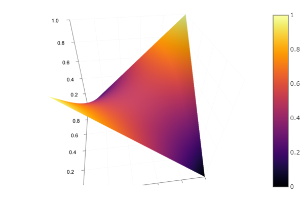
That final \(Z(P)\) equation finally maps some x and y coordinate to a z coordinate on our surface, meaning we can finally plot out our surfaces! The first example we'll look at is a trivial one: four points sampled from a plane. This should yield a simple solution. Specifically the four points we will use are \((0, 0, 0)\), \((0, 1, 1)\), \((1, 0, 1)\), and \((1, 1, 2)\). Plugging these four points in as A, B, C, and D in our equations as necessary, we get the following surface when plotted:

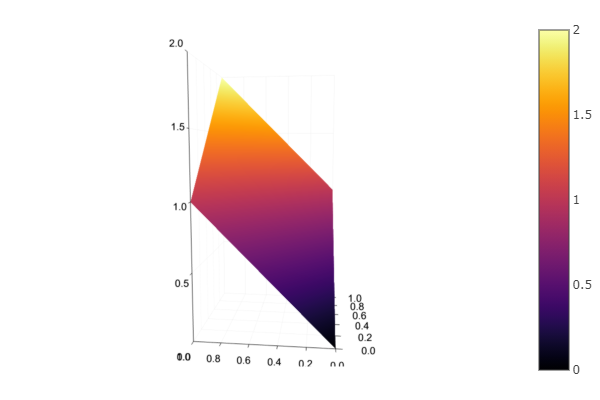
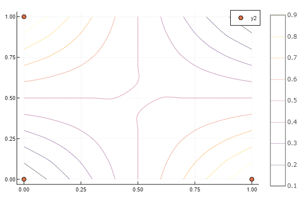
3D surface plots are often difficult to interpret, so here's the contour plot as well:

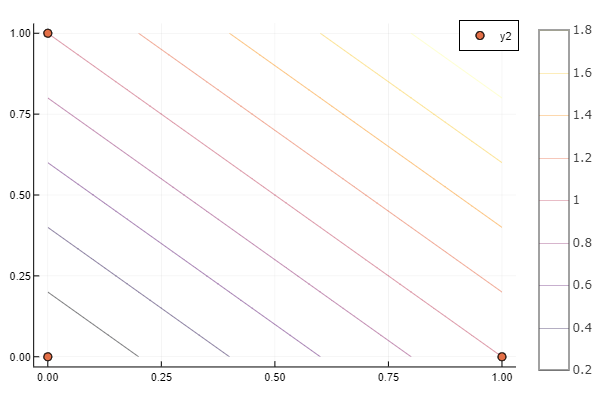
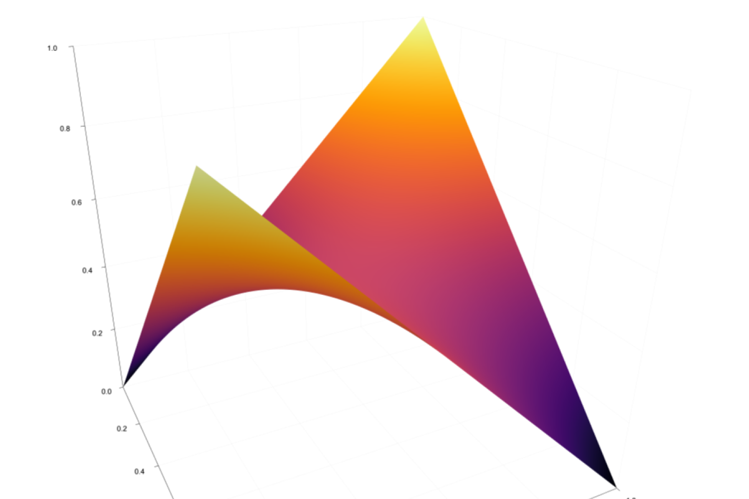
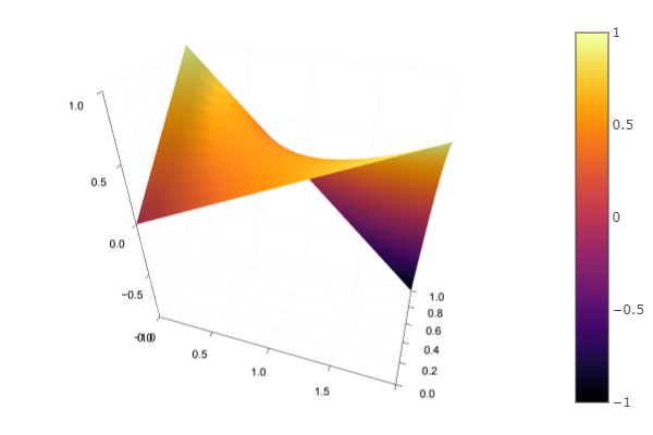
You can see that this plot is a simple plane, and that was to be expected with our choice of A, B, C, and D. But we wrote this function to work with points that cannot all be intersected with a simple plane. Let's use the same A, B, and C values, but change D to \((1, 1, 0)\). Now all four coordinates are the following: \((0, 0, 0)\), \((0, 1, 1)\), \((1, 0, 1)\), and \((1, 1, 0)\). If you picture these four points, you'll see that there is no way to draw a plane between all four of them, because point D is now too low, and they form a sort of saddle shape. So now let's see what the formulas produce:

You may be able to see the two higher points (B and C), which are in a yellowish color. Points A and D, however, are set to be at \(z=0\), and so their surrounding space is a dark bluish-black color. Once again the contour plot is a little easier to see clearly:

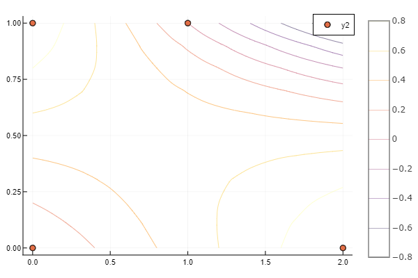
So what about situations where the points aren't perfectly placed in a square shape? Lets use the same Z coordinates, but instead we will place point C at the x and y coordinates of \((2, 0)\) instead of \((1, 0)\).

And the contour plot once again makes things more clear:

I really think these plots are remarkable! But to really get a feel for what's happening I've made a Pluto.jl notebook for generating these plots for yourself. I've written an article about installing Pluto.jl and making notebooks, so if you've never used it before but want to try out this math for yourself, I would advise checking out that article. To run my notebook, simply go to the main Pluto.jl page once you've downloaded it and enter in the following URL to open: https://gist.github.com/ctrekker/f50b8cc19fbd2c4cf54a9997e3393a2d.