A guide to building reactive notebooks for scientific computing with Julia and Pluto.jl

Julia is a fantastic language combining many of the higher-level features associated with Python with speed of C. Through JIT compilation, the language itself is dynamically typed but gets converted to statically-typed blazing fast machine code just before executing.
So what is a notebook, let alone a reactive one? When writing code in a file, each line or block of lines contains logic. In a notebook, each statement is contained in a notebook cell. This form of code is hugely common in the world of data science, and the most popular software for building them is Jupyter. Language bindings for virtually every language exists for Jupyter, including both Julia and Python. However, Jupyter notebooks execute sequentially, where one cell is considered dependent on all the cells above it. Although this format has been shown to work well in many circumstances, it falls short on a couple of fronts. These shortcomings are addressed with Pluto.jl and Julia!
So what does a reactive notebook do? In Pluto’s case, it keeps track of which cells depend on which other cells’ code, and can automatically re-execute each time a cell it depends on is updated. As we will discuss, this has a multitude of hugely advantageous properties. Straight off the bat, it means that notebook cells do not need to follow the order in which their code should execute. Instead you have free control over the flow of your notebook, giving you the liberty to reorder cells to make sense to the human reader rather than the computer one.
Installation
Installing Julia
The installation process for Pluto is made extremely simple with the built-in Julia package manager called Pkg. First though, we actually need to install Julia. Visit the Julia website and head to their downloads section. There are a multitude of different release types, but I recommend the latest stable edition. Select the appropriate platform for your computer and download the executable (or zip). If you choose to install Julia through an executable installation medium, the PATH environment variable will be updated for you automatically.
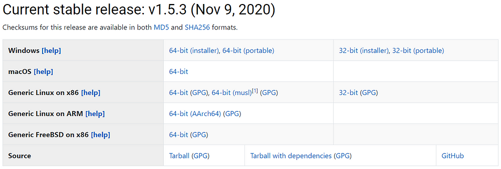
After installing Julia a new application should be present on your computer, in my case called “Julia 1.5.3”. At the time of writing this is the latest release, but major version 1.6 will be released soon. None of the steps for installation of Pluto will change in this release or likely any other nearby releases.
Installing Pluto
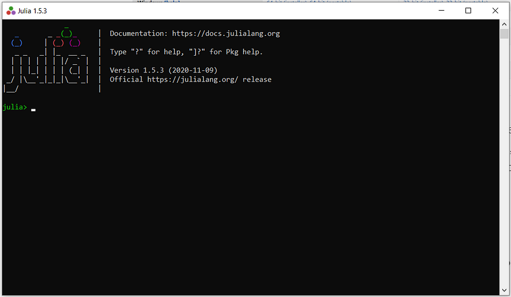
Open up the Julia application. For me that’s “Julia 1.5.3”. Your computer should open up a command-line looking application. This interface is called the Read-Eval-Print-Loop (REPL for short). Below is an image for what it looks like for me:
Inside this command interface, type the character ]. This should make your REPL interface switch to package manager mode, which looks like this:
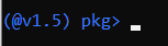
From here simply type add Pluto, which will download the Julia package registry and the latest version of Pluto. Note that if this is your first time using the Julia package manager then it could take a couple of minutes for initial setup to happen.
Once Pluto installation has finished and your REPL prompt looks like it did before you added Pluto, press Backspace to exit package manager mode. The REPL prompt should turn green, meaning we are now ready to start Pluto.
Starting Pluto
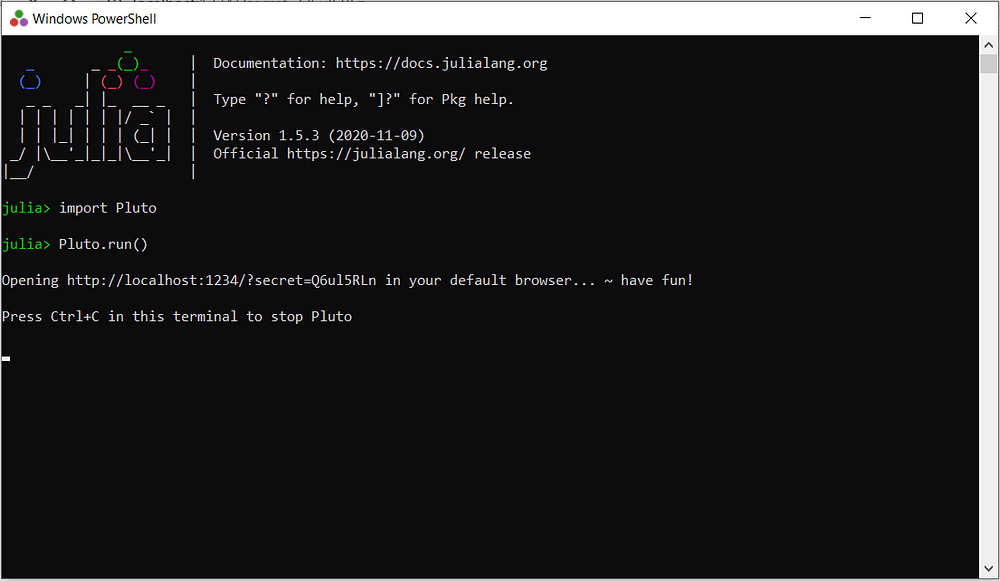
This part is really simple. Open up a Julia REPL prompt if one isn’t open already. Ensure that the prompt is green, meaning it is in Julia code execution mode. Type in import Pluto, then press enter. You should get a message after precompilation has completed instructing you on how to start a Pluto server. Now, type in Pluto.run() and press enter. This will start a Pluto server on port 1234 and open it in your default browser. Now we’re ready to start writing reactive notebooks!
Making our first notebook
The Basics
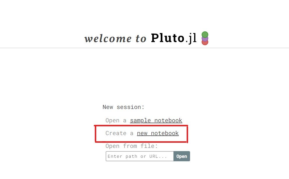
Lets get started with an empty notebook. Click on the “Create a new notebook” link (shown below) to create a new, blank notebook.
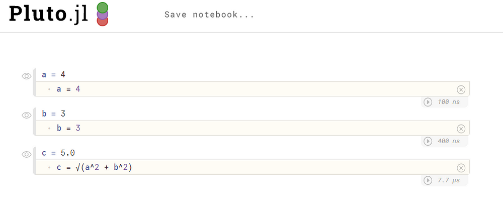
An interface which may feel familiar if you have experience with Jupyter notebooks should appear after it finishes loading. Lets try writing some code in these cells. If you don’t know Julia, no worries! The code I present here will work, and you’ll pick up Julia quickly if you already know Python. In the first cell, enter the following code: a = 4, and press control (or command) + enter. This will submit the changes and add a new cell below. For reference, shift + enter will submit the changes and execute the code without adding another cell below. In the cell below, add b = 3 and do control + enter again. In the final cell, enter c = sqrt(a^2 + b^2), and the result (shown above each cell) should be 5.0.
On a quick sidenote, Julia supports Unicode characters, meaning a function with the name √ can be defined. Indeed, the square root function is defined by default as both sqrt and √. To insert a √ character, type \sqrt and then press tab inside one of the code cells. The code works exactly the same if instead of sqrt we use √ (now mine looks like c = √(a^2 + b^2)).
Reactivity
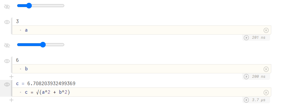
Lets go ahead and try out the “reactive” part of Pluto now. Try to change the value of a from 4 to something else (like 5). Then press shift + enter to update the code. You should see that the c value has reacted to that change and been updated! If you changed a to 5, c ≈ 5.83. This is the main beauty of Pluto notebooks. With Jupyter notebooks, each cell would have needed to be re-executed individually. With Pluto, however, dependencies between cells are known and can therefore intelligently update the notebook cells which depend on the cell being updated, all in the proper order!
Interactivity
So what about the nicer user inputs like sliders or text boxes? These work out-of-the-box with Pluto using a Julia macro called bind. Its super simple to use, so lets change our code to work with sliders.
In the cell which defines the variable a, change the code to match the following:
@bind a html”<input type=’range’ min=’1' max=’10' step=’0.25'/>Do the same for the cell defining b, but replace the “a” after the “@bind” macro with the letter “b”.
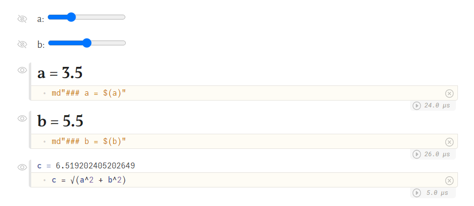
Now you should see 2 sliders. Try dragging them around, and you should see the value of c change correspondingly. There is one problem though: the values of a and b aren’t actually displayed anymore. Lets fix that. Below the value bind for a, add a cell with the plus button which appears, and simply type “a” into it. Then run it. You should see the value of a appear, and will change accordingly each time you drag the slider. Do the same for b. Then click the little eye icon next to each of the bind cells. This will make their code disappear, as their code is irrelevant in relation to the Pythagorean Theorem. My notebook now looks like this:
Markdown is also supported natively, which looks like this:
Above and Beyond
The demonstration I walked through above was rather trivial, so lets do a more interesting one now. Lets make an interactive plot!
To make plots, we need the “Plots” Julia package. This can either be installed in a similar manner to what was done for Pluto, or it can be done within the Pluto notebook itself using two cells, each one corresponding to the two lines below:
import Pkg
Pkg.add("Plots")
This will take a bit to install, but once it has been installed these two cells can be deleted. Next up, we have to include plots in our notebook with a cell containing the following:
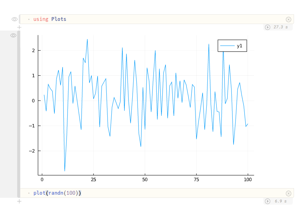
using PlotsAs an example, we can plot random numbers with the notebook configuration shown below.
This can be combined with interactivity to create an interactive plot! In the following demo, I use a slider to define the phase shift of a sine wave. I then plot the phase-shifted sine wave, a standard sine wave, and the sum of these two waves.
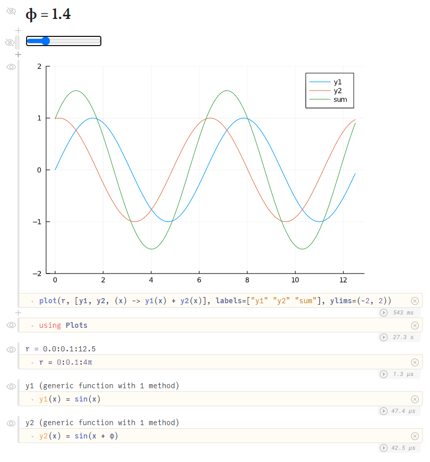
Notice how the cells are not in sequentially executing order. The import of Plots comes after the plot, and the functions that are being plotted are defined at the end! With Pluto it doesn’t matter what order you put the cells in, leaving the author the freedom to optimize human readability rather than computer readability. In this case, the point was to showcase a simple interactive plot, leading me to put the showcase at the top and the code that makes it work below it.
Conclusion
Pluto notebooks make building interactive code with Julia so much more intuative and has proven to be a valuable tool in data science and research with Julia. By no means will it eradicate Julia in Jupyter notebooks. Jupyter notebooks still have their place and will for a long time. However, Pluto addresses some of the main problems, and uses the powerful language of Julia to do so. It is completely open-source, available at https://github.com/fonsp/Pluto.jl, and is powered by Julia itself. I look forward to seeing the beautiful notebooks you will create!