Working with stock market data using Robinhood Stocks and Python

I've always loved writing market analysis programs. A couple years back I used a free API called AlphaVantage. AlphaVantage still exists, but with the decline in popularity of trading commissions, the opportunity for programatic analysis and even trading has skyrocketted. Some would attribute this trend to Robinhood's commitment to commision-free stock trading, forcing the competition to adopt lower or zeros commission stock trading. Today we will explore building a Python application that views historical data and does some rudimentary analysis. To do this we will utilize Robinhood's completely free API. No official documentation exists, but plenty of community-made documentation and libraries exist for interfacing with it.
Getting Started
Environment Setup
For this project we will be using Python. There are several reasons for this. Firstly, a plethora of data science libraries exist for Python already, which will make analysis easier. Secondly, a community-built library for interfacing with the Robinhood API already exists.
Let's start by making a fresh Python environment, so open up your terminal! We'll be calling this project robinhood-market-analysis, so we'll start by making a new directory with this name.
mkdir robinhood-market-analysis
cd robinhood-market-analysis
Now we have to create a virtual environment for Python. The command below will create a new virtual environment based on the Python version located in your PATH environment variable. The .venv parameter in the command is the location the virtual environment will be placed. In this case, a new folder called .venv will be created in the working directory.
python -m venv .venv
Next, lets activate the virtual environment. This means that we will switch our Python installation from the globally installed version to our local virtual environment version.
.\.venv\Scripts\activate.batIf you aren't on Windows, the above won't work. Rather, the command below will activate the new virtual environment
source .venv/bin/activate
Now when new packages are installed, they will be installed in the virtual environment rather than the global Python installation. This has numerous advantages which will not be discussed here, but if you're curious check out this article.
To wrap up our environment setup we need to create a requirements.txt file. This will list our dependencies and their target versions, making the project more reporducable and makes installing dependencies easier.
We will be using robin-stocks to download market data using the Robinhood API, pyyaml to parse configuration files, and pandas for storing and querying market data using a DataFrame.
robin-stocks==1.5.4
pyyaml==5.3.1
numpy==1.19.4
pandas==1.2.0
matplotlib==3.3.3
mplfinance==0.12.7a4Then, to install the dependencies listed in requirements.txt, we run
pip install -r requirements.txtNow our Python environment is set up for making our market analytics program!
Version Control Setup
For this project I'll be using Git. If you don't plan on sharing this project with anyone else or simply don't see the need for version control based on your needs, skip this step. Since I am publishing this project on GitHub, git is a necessary piece of this project.
git initNow we need a .gitignore file to prevent Git from tracking the virtual environemnt files. These files are platform-specific and it is up to those who clone the repository to make their own virtual environment if they see fit. We will be adding more to this file later.
.venv/Let's create our initial commit now.
git add .gitignore
git add requirements.txt
git commit -am "Initial commit"
If you want to publish your project on GitHub, then add a new remote for it.
git remote add origin https://github.com/ctrekker/robinhood-market-analysis
git push --set-upstream origin master
Authenticating with Robinhood
Before we can download and parse market data, we have to authenticate with Robinhood. To do this you need to create an account with them if you haven't already. Making an account is completely free, but is limited to United States residents and those over 18.
To start, we need a Python file we can run to authenticate with Robinhood. We will call this file auth.py. That way, whenever we want to authenticate with Robinhood, we only need to include this file rather than rewrite the same code over and over.
import robin_stocks as rs
import yaml

with open(r'credentials.yaml') as configFile:
    config = yaml.load(configFile, Loader=yaml.FullLoader)

rs.login(username=config['username'], password=config['password'], expiresIn=86400, by_sms=True)

print("Authenticated with Robinhood")This will load your Robinhood account credentials from the credentials.yaml file and use them to log into the Robinhood API. As of now the Robinhood API does not support token authentication, so we have to use our account credentials (basic authentication) instead. Your first time running this code (with python auth.py), the program will prompt you for an SMS code sent to verify this device. Once you enter this once Robinhood will remember the device and the program will run without any user input.
username: <ROBINHOOD-USERNAME>
password: <ROBINHOOD-PASSWORD>If you are using version control such as Git for this project, make sure not to commit credentials.yaml!! This file contains your username and password, which means if anyone were to gain access to your version control repository they would also be able to gain access to your Robinhood account. To prevent accidental addition of this file to version control, add a line containing credentials.yaml to your .gitignore file (if using Git).
Downloading Market Data
Now it's time to use the Robinhood API to download some market data. Depending on what you want to do, you can download historical data or realtime stock data. I'll be going over how to download historical data. To go further, check out the robin-stocks documentation to see the full list of functions that can be called to retrieve data.
Historical Data
We will start by making a new file called historical.py. When we want to download historical stock data we can simply run python historical.py within our virtual environment.
First we need to include the necessary libraries for the file
import robin_stocks as rs
import pandas as pd

import auth # Runs our auth file so we are authenticated with RobinhoodNext we need to create yet another file containing a comma-separated list of stock symbols we want to query. Below is a sample file that I'll be using for the rest of this guide, but feel free to add or remove any symbols you like.
ARCT, SPCE, CPRX, BABA, AMZN, SNE, APHA, GOOGL, MSFT, NRZ, PLUG, PTON, NKE, FB, GM, KO, UBER, MRNA, ZNGA, TXMD, LI, JNJ, RCL, WMT, DKNG, AZN, PENN, SNAP, GE, ET, NOK, BP, DAL, LUV, DIS, SIRI, NFLX, NVDA, BAC, AAPL, NIO, OGI, PFE, SQ, ADT, SBUX, ZM, KOS, PLAY, UAL, SAVE, AMD, BA, NCLH, HAL, HL, T, JBLU, WFC, MRO, INO, RKT, TSLA, CRON, TWTR, CGC, MGM, AAL, GPS, F, GPRO, ACB, MFA, TLRY, CCL, XOM, COTY, AM, M, AMC, FIT, NKLA, GNUS, PSEC, GUSH, WKHS, PLTR, IVR, IDEX, FCEL, UCO, USO, VOO, ABNB, SPY, SRNE, KODK, SOLO, XPEV, VXRTSince we will use this list of symbols for downloading historical data as well as analyzing it, we should make a new file called symbols.py that we can include in both historical.py and later in our analysis scripts.
import re

with open('symbols.csv', 'r') as symbols_io:
symbols = re.split(r',\s*', symbols_io.read())Then add an import statement to historical.py to include the list of symbols in the file.
from symbols import symbolsNow that we have the list of symbols we want to query, we can actually query some historical data! The function stocks.get_stock_historicals does accept either a list of symbols or a single symbol. However, only a certain amount of entries are allowed to be queried at a time, meaning the smaller the interval and larger the span is, the fewer symbols can be queried at a time. We want our program to be able to support any interval or span supported by the API itself, so we will query each symbol individually.
interval, span = 'day', 'year'
historical_data = {}
failed_symbols = []

COLOR_GREEN, COLOR_RED, COLOR_CYAN, COLOR_END = '\033[92m', '\033[91m', '\033[96m', '\033[0m'
for symbol in symbols:
    try:
        historical_data[symbol] = rs.stocks.get_stock_historicals(symbol, interval=interval, span=span)
        print(f'{COLOR_GREEN}✓ {symbol}{COLOR_END}')
    except KeyboardInterrupt:
        exit()
    except:
        print(f'{COLOR_RED}✕ {symbol}{COLOR_END}')
        failed_symbols.append(symbol)
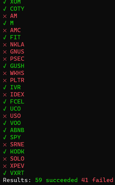
print(f'Results: {COLOR_GREEN}{len(symbols)-len(failed_symbols)} succeeded{COLOR_END} {COLOR_RED}{len(failed_symbols)} failed{COLOR_END}')Most of this code is fairly standard. You can see we define an empty dictionary to store each of the symbols' historical data on line 2, and try to query each symbol and add it to that dictionary. However, if the user wants to exit the program early by using a keyboard interrupt, we catch the exception on line 10 and exit the program. If an unknown error occurs, we assume there was a problem querying the data and print an error message and add the symbol to the list of failed symbols.
You may have noticed on line 5 we define some constants prefixed with COLOR_. These constants when inserted into a string will color the text in certain terminals. As you can see on line 9, we begin by inserting COLOR_GREEN to begin the green-colored section of the text. Then we insert the symbol, and end the string by inserting the COLOR_END constant, which signifies the end of a colored region. The same goes for lines 13 and 16. I'm using the Windows Command Prompt and the coloring works properly. I have tested this on Linux as well, and coloring works there as well. I haven't tested on MacOS, but I suspect it would work the same as it does on Linux terminals. You can see below a portion of this output in my command prompt window. The large amount of failures is caused by purposefully-raised exceptions with random numbers to demonstrate the error-catching system. In an ideal setting these queries will rarely if ever fail.
Now we have one more thing left to do: save all the historical data we downloaded to a file we can read later for analysis. We will be using Pandas DataFrame to do this.
dataframe_file = 'historical.csv'

historical_formatted = {}
for symbol in  historical_data.keys():
    symbol_data = historical_data[symbol]

    for symbol_entry in symbol_data:
        for symbol_entry_key in symbol_entry.keys():
            if not symbol_entry_key in historical_formatted:
                historical_formatted[symbol_entry_key] = []
            historical_formatted[symbol_entry_key].append(symbol_entry[symbol_entry_key])

historical_df = pd.DataFrame(historical_formatted, columns=list(historical_formatted.keys()))
historical_df.rename(columns={'open_price': 'Open', 'close_price': 'Close', 'high_price': 'High', 'low_price': 'Low', 'volume': 'Volume'}, inplace=True)
historical_df.to_csv(dataframe_file)
print(f'Saved to {COLOR_CYAN}{dataframe_file}{COLOR_END}')This code reformats the data returned from each of the historical_data entries into a format acceptable by pd.DataFrame. It loops through each of the symbols in historical_data, loops through each of the symbol data entries, and adds each key/value to its corresponding list inside historical_formatted. Then a DataFrame is created from the formatted historical data and save to the file path set in the variable dataframe_file. And that's it for historical.py.
The full code for historical.py can be found here, in the GitHub repository for this article.
Analyzing our Data
Obviously after the data is saved you can go as far as you like in analyzing it. The examples below are not meant to be the only or correct way to perform analysis. Rather the code below should serve as an example to get started from. Ultimately this step is largely up to you to implement yourself.
Visualization
Let's start by creating a new Python file for generating visualizations of our data. The new file will be called historical_vis.py. We saved our downloaded historical data to historical.csv, so we will start by loading it back into a Pandas DataFrame with the following code:
import pandas as pd
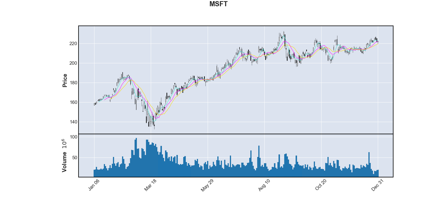
historical_data = pd.read_csv('historical.csv')Now we can visualize our data with matplotlib and mplfinance. The mplfinance package has a function called plot. This function takes in lists of open, close, high, and low values (hence ochl) and plots them as a candlestick plot. This function conveniently takes in a DataFrame object, but requires the column names for open, high, low, close, and volume to be Open, High, Low, Close, and Volume respectively. We also have to configure our DataFrame to have its index be the begins_at datetime object. The code segment below reconfigures the DataFrame inplace and plots a candlestick plot for MSFT (Microsoft). The mav keyword argument also tells plot to calculate and display 3 different moving averages. One with interval 5, another with 10, and another with 15.
historical_data['begins_at'] = pd.to_datetime(historical_data['begins_at'])
historical_data.set_index('begins_at', inplace=True)

import mplfinance as mpf
mpf.plot(historical_data.loc[historical_data['symbol'] == 'MSFT'], title='MSFT', type='candle', volume=True, mav=(5, 10, 15))
Here is the plot this code generates (at the time of writing):
It would be nice if our script automatically exported these plots to PNG files for every symbol we have in our list. To do this, we simply have to put the plotting line above in a for loop iterating over each symbol, and change the plot call a little bit to save to a file rather than display it in a GUI.
import mplfinance as mpf
from symbols import symbols
import os

if not os.path.isdir('historical_plots'):
    os.mkdir('historical_plots')

from colors import COLOR_GREEN, COLOR_RED, COLOR_CYAN, COLOR_END
s = 1
for symbol in symbols:
    progress_str = f'{COLOR_CYAN}{s}/{len(symbols)}{COLOR_END}\t'
    try:
        mpf.plot(historical_data.loc[historical_data['symbol'] == 'MSFT'],
            title='MSFT',
            type='candle',
            volume=True,
            mav=(5, 10, 15),
            savefig=f'{os.path.abspath(os.getcwd())}/historical_plots/{symbol}.png')
        print(f'{progress_str}{COLOR_GREEN}✓ Plotted {symbol}{COLOR_END}')
    except:
        print(f'{progress_str}{COLOR_RED}✕ Plot failed for {symbol}{COLOR_END}')
s += 1This iterates over every symbol and saves its candlestick plot inside a historical_plots folder in the working directory. Its program output is similar to to that of the download process. A screenshot of some of its console output is below:
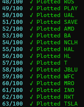
historical_vis.py Console Output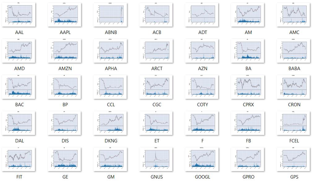
historical_plots folderStatistics
As a simple example, one may want to extract some summary statistics of the historical data. To do this, Pandas includes some nifty methods on DataFrame objects that will calculate these. We'll start once again by making a new file called historical_stats.py. This will contain our code for calculating and displaying our summary statistics of our historical data.
To start we will include Pandas and import our data as we did for visualizations.
import pandas as pd

historical_data = pd.read_csv('historical.csv')As an example we will look at the summary statistics for Tesla (TSLA) from December 1th to December 31th of 2020.
symbol = 'MSFT'
start_date = pd.to_datetime('2020-12-1 00:00:00+00:00')
end_date = pd.to_datetime('2020-12-31 00:00:00+00:00')
selected_data = historical_data.loc[(historical_data['symbol'] == symbol) & (historical_data['begins_at'] >= start_date) & (historical_data['begins_at'] <= end_date)]
print(selected_data.describe())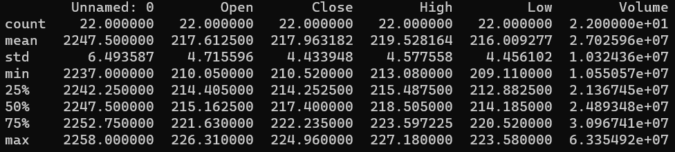
These summary statistics aren't particularly useful in describing more than the general state of a particular stock, but this strategy is not limited to the basic statistical parameters. The describe method of a DataFrame instance will calculate these parameters1. To calculate parameters more relevant to market data, you can define your own functions which reduce an input DataFrame to a table similar to the one above with rows for each parameter.
Conclusion
From here on out the mechanism for obtaining stock data in a convenient form is at your fingertips. Often times I find that obtaining the data in a proper format for analysis is half the battle. The visualizations and statistic calculations performed in this article are but the tip of the iceberg in the vast worlds of Data Science and Finance. If you're someone like me, being able to see and manipulate the data with your own hands (or more accurately your own code) helps greatly in learning about it on a deeper level. I would much rather build my own tool for evaluating whether a stock is good to buy or sell than simply take the word of others for a few reasons. For one, there is always room for selfishly motivated advice, especially when money is involved. Secondly, taking someone else's advice isn't necessarily always bad, but it can take away the opportunity to learn firsthand why a decision is made. It's just as the proverb written by Lau Tzu teaches: "Give a man a fish and you feed him for a day. Teach a man to fish and you feed him for a lifetime"2.
Footnotes
[1]: https://pandas.pydata.org/docs/getting_started/intro_tutorials/06_calculate_statistics.html